The cool thing about looking at a signal in the Frequency Domain is that you can do all sorts of things to the signal that would be a lot harder to do in the time domain. For example, you could filter it. 

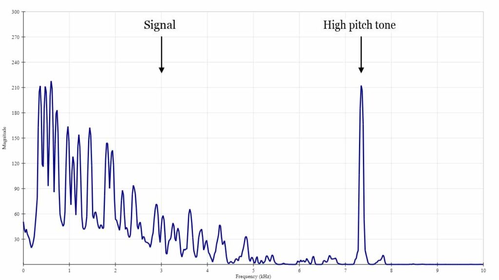
Here’s a signal, a nice musical chord, but it has an annoying high-frequency squeak on it that I want to get rid of.

If I look at the signal in the frequency domain, I can clearly see the high pitch squeak.

To remove the squeak, I need to multiply all the frequencies I want to keep by 1, and all the frequencies I want to get rid of by 0.

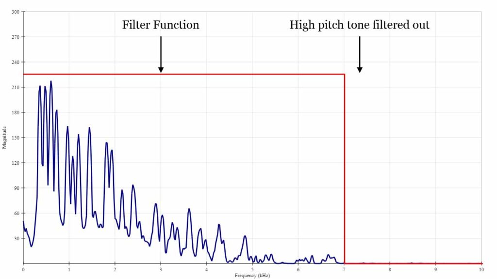
Then I can convert the signal back into the time-domain, and hey-presto, I have a nice clean signal.

But converting the signal into the frequency domain using the Fourier Transform, applying the filter, and then using the Inverse Fourier Transform to convert the filtered signal back into the time domain, sounds like a lot of work. Is there any way we can perform the whole operation in the time domain?

Yes, there is! “A multiplication in the frequency domain is a convolution in the time domain.”

Let’s look at what that means and how we can use our knowledge of the Fourier Transform to build a Finite Impulse Response filter.

What is Convolution?

If you’ve ever performed a moving average on a set of data, you’ve performed a convolution. Moving averages are sometimes called running or rolling averages, and are used a lot in financial markets to identify trends from volatile daily data.

How does a moving average work?

Let’s begin with some noisy data shown on the graph below.

You take your data and draw a window around the first few lines. For example, your data may contain 250 lines and you might draw a window around 25 of them. You then take the average of all the data points in the window..

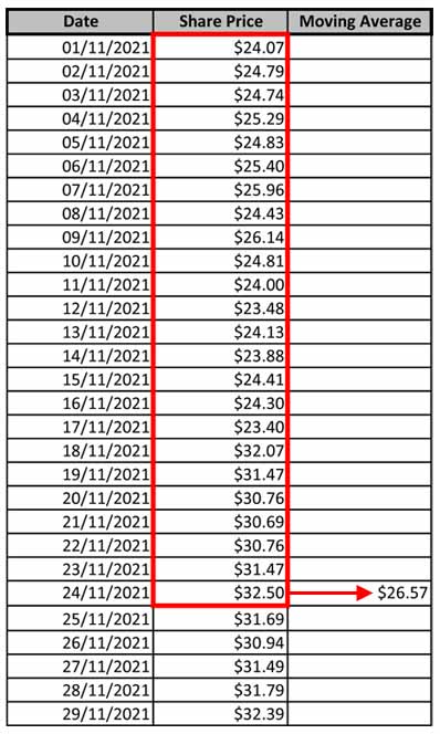
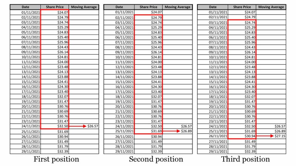
Then, you move your window down the list by one line and take another average.

You continue doing this until the window reaches the end of your data. The first 3 steps of this process are shown below.

When you plot the graph of the moving average data, it looks like this:

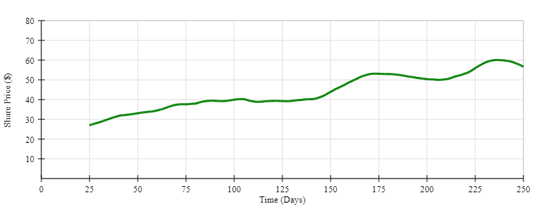
The line is a lot smoother. It’s as if you have applied a low-pass filter to the data. In fact, that is exactly what a moving average is: a kind of crude low-pass filter that we calculated by performing a convolution.

The formal definition of convolution

Convolution is defined as: “the integral of the product of two functions after one is reversed and shifted,” and is expressed mathematically as follows:

$$ (f * g)(\tau) = \int_{-\infty}^{+\infty} f(t) \times g(\tau – t) \cdot dt $$

In the equation above, we have 2 signals: f(t) and g(t). In our moving average example, f(t) is the financial data we began with. g(t) is the signal we convolved that data with. g(τ-t) simply means that g(t) has been shifted along the x-axis by an amount of time equal to τ. As τ changes, g(t) moves further along the x-axis. But what does g(t) look like?

To compute an average, we add all the data points in the window together, then divide that sum by the number of data points in the window. We then keep moving the position of the window and calculating the average of its contents for each new position.

Now let’s convert this idea into the terms of a convolution. The moving average is like convolving the signal, f(t), with a rectangular function. So, g(t) is a rectangular function.

The width of g(t), which I’m going to call, N, is equal to the number of data points we are averaging each time. It performs the summing part of the averaging operation. The height of g(t), which will be \( \frac{1}{N} \), performs the dividing part of the averaging operation on each sample.

You can see this process graphically below. (Note: The height of g(t) is not to scale)

Notice how the output of the convolution is delayed. The green line doesn’t start until 25 days. This is because the moving average has to accrue 25 days worth of data before the first average can be taken. This phase delay is a common feature of all filters and is a consequence of the filtering process.

The frequency response of a moving average filter

So we’ve discovered that the moving average acts like a sort of low-pass filter, but what is its frequency response? Is it anything like the nice, sharp rectangular shape we are trying to achieve?

To find the answer, we need to perform a Fourier Transform on g(t). I won’t do the actual math for the Fourier Transform of g(t) just yet. There will be ample opportunity for that in the next post. I’ll just show you what the frequency response of the moving average filter looks like.

As we see from the graph, the higher frequencies are attenuated, but it’s not the nice sharp rectangular shaped function we set out to design. What can we do to g(t) to turn it into the sort of function that will give us the frequency response we are looking for?

Clue: “A multiplication in the frequency domain is a convolution in the time domain” and vice versa.

We’ll find out in the next post.