How FIR filters work | Making a practical filter

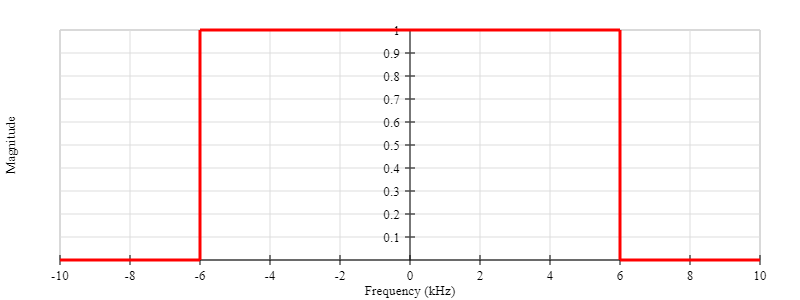
In the last post, we calculated the kind of convolving function that would give us the frequency response we were looking for in our low-pass filter (shown below).
The convolving function we calculated, \( g(t) \), looks like this:

\( g(t) \) is known as the impulse response of the filter. The impulse response of a filter tells us how the filter would react if it were presented with a brief input signal, called an impulse. An impulse is an infinitely tall, infinitely thin vertical line.
There are a number of problems with this filter that prevent us from being able to implement it in the real world.
- The impulse response is not defined at time, t=0.
- This filter is not causal.
- We are working with digital signals.
1. The impulse response is not defined at time, \( t=0 \)
If we plug \( t=0 \) into the equation for \( g(t) \), we find that \( g(t=0) = NaN \). This is because, when \( t=0 \), we are dividing by zero. You may recognize the shape of the impulse response as a sinc function which is defined as:
$$
sinc(x) = \begin{cases}
\frac{sin(x)}{x} & \text{ if } x \neq 0 \\
\;\;\;1 & \text{ if } x = 0 \\
\end{cases}
$$
So if we use a sinc function to describe the impulse response of our filter, we can ensure that it is defined for all values of time. However, if we simply replace \(x\) by the contents of the sine expression, we get:
$$ sinc(2\pi f_c t) = \frac{sin(2\pi f_c t)}{2\pi f_c t} = \frac{g(t)}{2f_c}$$
Therefore, we have to multiply by \( 2 f_c \) to make it equal to \( g(t) \).
$$ g(t) = 2f_c \cdot sinc(2\pi f_c t) $$
This means that:
$$
g(t) = \begin{cases}
\frac{sin(2\pi f_c t)}{\pi t} & \text{ if } x \neq 0 \\
\;\;\; 2f_c & \text{ if } x = 0 \\
\end{cases}
$$
Now we have an impulse response that is a function of the cutoff frequency of the filter. In the demonstration below, use the slider to change the cutoff frequency of the filter to see what it does to the impulse response.
2. This filter is not causal
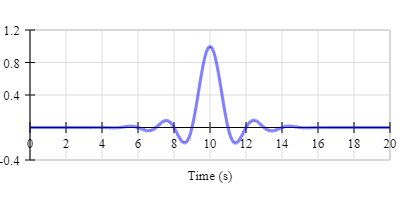
A filter is said to be causal if its output is the result of only current and past inputs. In the real world, no filter can know that it is about to receive a sudden impulse before that impulse arrives. However, if you look at the impulse response graph for this filter, the filter starts reacting to the signal BEFORE the signal is received at t=0. As it stands, this filter is NOT causal and cannot exist in the real world. We, therefore, need to shift the impulse response along the x-axis so that the filter starts reacting to the signal only after the signal has been received at t=0. Unfortunately, this is not so easy to do.
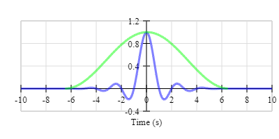
The impulse response of this filter is infinite. In other words, it goes on forever. Notice how the little wobbles on either side of the main peak of the impulse response never totally settle down.
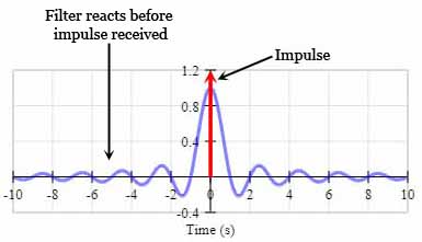
Just as the wobbles on the right-hand side of the graph decay forever after t=0, so the wobbles on the left-hand side have been building forever since the beginning of time, reaching a peak at t=0.
To be able to shift the impulse response along the x-axis and make this into a causal filter, we need to know where the impulse response starts. However, we just said that the impulse response has been building since the beginning of time. It doesn’t have a start. It is infinite.
Therefore, we are going to have to somehow turn this filter into a Finite Impulse Response (FIR) filter so that the impulse response of the filter will last only for a finite amount of time.
This is going to have a detrimental effect on its frequency response, so the filter will no longer give us the perfect box-car shape response we designed. However, we have no choice. We’re going to have to make a good old engineering compromise. On the one hand, the longer we give the filter to settle down, the closer its response will be to the ideal filter we set out to design. But on the other hand, truncating the impulse response means an easier calculation, less memory needed to store the samples, and a shorter delay from the moment the input is received, to the moment we see an output.
For the purposes of this demonstration, I’m going to arbitrarily truncate the impulse response at 6.5s. I could simply chop the signal at ±6.5s. However, this causes an ugly discontinuity in the impulse response at ±6.5s.
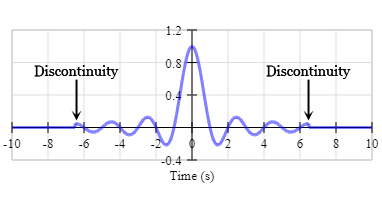
A cleaner way to do it would be to smooth the truncation using a windowing function like a Hanning window (shown in green). Remember, whatever window we use is going to affect the frequency response slightly. As we’ll see shortly, using a windowing function can actually improve the frequency response, making it smoother both in the pass and stop bands of the filter.
Now we can shift the impulse response along the x-axis and make the filter causal.
3. We are working with sampled signals
All the graphs above, display a continuous-time signal impulse response. This is not the case with digital signals. Digital signals are sampled; time is discrete. Therefore, there are a number of changes we have to make to the way we calculate \( g(t) \) to account for their sampled nature.
Discrete Time
We have to change the continuous variable, t, in our equation into a discrete, n, where n = 0, 1, 2, etc. This means that there will now be a finite number, N, of points in our impulse response. In the world of digital filters, these points are known as taps.
The sampled nature of the impulse response will also have an effect on how we express the cutoff frequency of the filter.
Normalizing the cutoff frequency
When we defined this low pass filter, we set the cutoff frequency, \( f_c \), to 6 kHz to get rid of the 8 kHz squeak in my signal. However, my signal is digital. It was sampled at 44.1 kHz. So the cutoff frequency must be normalized to the sampling frequency, \( f_s \). I’m going to call this normalized cutoff frequency, \( f_t \), such that:
$$ f_t = \frac{f_c}{f_s} $$
For my filter:
$$ f_t = \frac{6}{44.1} \approx 0.14 $$
Making the filter causal
We have to shift the impulse response along the x-axis to make the filter causal. There are N taps in this filter. So to shift the impulse response so that it begins at t=0, we have to shift it by \( \frac{N}{2} \) samples. Therefore, our discrete-time variable, n, becomes:
$$ n \rightarrow n – \frac{N}{2}$$
This is going to introduce a phase delay into the filter’s impulse response. After all, the filter cannot begin to react until it has an input to react to, and that reaction takes time.
Phase delays are nothing new with filters. They are a consequence of the filtering process both in digital and analog filters. However, one distinct advantage of FIR filters is that the phase delay is the same for every frequency. This is not the case with any other type of filter, including analogue filters.
Ensuring there is a center point
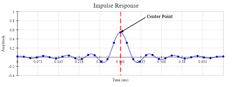
The graph above shows the impulse response of a low-pass filter. The dark blue points are the taps. The impulse response peaks in the middle and is symmetrical about this center point. This is an important feature of the filter, so we want to ensure that there is a tap at this center point. Therefore, we make sure that there are always an odd number of taps in our FIR filter. For example, there are 33 taps in the above filter.
Shifting the impulse response along the x-axis, and ensuring there is a tap at the center point, means we have to further modify our discrete-time variable, n, which becomes:
$$ n \rightarrow n – \frac{N-1}{2}$$
So the impulse response equation for our digital low-pass filter is now:
$$
g_n = \begin{cases}
\frac{sin(2\pi f_t \left (n-\frac{N-1}{2}\right ))}{\pi \left ( n-\frac{N-1}{2} \right ) } & \text{ if } n \neq \frac{N-1}{2} \\
\;\;\;\;\;\;\; 2f_t & \text{ if } n = \frac{N-1}{2} \\
\end{cases}
$$
Filter Demonstration
In the demonstration below, you can design a low pass filter to filter the noisy signal we met in the introduction to this series on FIR filters. The demonstration has 3 sections.
In the first section, press play to hear the noisy signal and see it represented on the time domain and frequency domain graphs. Once you have listened to the noisy signal, scroll down to the second section to design the filter.
In the second section, you can design a filter to try and get rid of the high pitch squeak in the the signal. Play with the cutoff frequency, the number of taps and the windowing function to try and get the best response. The frequency response graph in the filter section shows the desired box-car shaped response in red, the frequency response of the filter you designed in green.
You can then test your filter out by pressing the “Test Filter” button. This will play your filtered signal so you can see and hear the results of your filter.
In the third section, you can see the values of the individual taps in your filter as well as all the equations used to calculate them.
Applying the filter
So we’ve designed our filter and we know what it’s impulse response looks like. Now we need to apply it to a sampled signal. How might we perform the filtering process in code which you can run on your computer?
Clue: An FIR filter is simply a weighted running average.
We’ll find out in the next post.

